
I co-founded Precision Analytics with Erika, also holding a PhD from McGill and am an accredited statistician. While overseeing our …
A gentle INLA tutorial
INLA is a nice (fast) alternative to MCMC for fitting Bayesian models. They each have some pros and cons, but while MCMC is a pretty intuitive method to learn and even implement yourself in simple scenarios, the INLA algorithms were a mathematical stretch for me.
I think it’s better now, but when I was first learning INLA for my dissertation, there weren’t a ton of gentle introductions. I spent months during my PhD going over and over the proofs in the seminal INLA paper, trying to make sense of it all.
For my own benefit, I put together a summary that was intended for an applied statistician – someone like me, familiar enough with theory like the normal distribution, Taylor series expansions, and Bayes theorem, but who maybe hasn’t spent a lot of time with the Hessian recently.
This is a really simplistic explanation; the seminal papers are really thorough and clear and are worth a read (or fifty) if you are interested in a more serious understanding. The details are interesting and important. But this is my attempt at giving you the ‘gist’ and it’s something I wish I had when I was starting.
Hierarchical models are widely used across disciplines to represent complex dependency structures in data. Uncertainty in model parameters and latent variables or processes can be encoded with appropriate prior distributions using a Bayesian framework.
While there is almost never a closed-form solution for the posterior distribution, general solutions via Markov-chain Monte Carlo (MCMC) methods have been developed into software like WinBUGS. MCMC is slow, does not scale well, and for some complex models can fail (model will not converge). Newer software (JAGS, Stan) have tried to address these challenges.
MCMC is an asymptotically exact method whereas INLA is an approximation. Sometimes use of INLA will be met with suspicion or questions like “But what about the approximation error? How confident are you in your results?” There are times where INLA will fail, but it’s good to remember that we don’t live in asymptopia. Empirically, the MCMC error and INLA error are frequently very similar, as has been shown in many simulation studies and I have observed myself many times.
INLA is a fast alternative to MCMC for the general class of latent Gaussian models (LGMs). Many familiar models can be re-cast to look like LGMs, such as GLM(M)s, GAM(M)s, time series, spatial models, measurement error models, many more.
To understand the gist of what INLA is doing, we need to be familiar with:
- Bayesian inference
- Latent Gaussian models (LGMs)
- Gaussian Markov Random Fields (GMRFs)
- Laplace approximations
If you’re interested in learning about INLA then I assume you are already familiar with Bayesian inference, but we’ll start with an extremely brief refresher.
In a Bayesian model, we generally want posterior distributions for our models (e.g., the distribution of the parameters given the data), or predictive posterior distributions (for prediction/forecasting – the distribution of new values given the observed ones). Let’s focus on the former case, the latter follows logically.
The posterior distribution is equal to the data likelihood multiplied by the priors over the normalizing constant (so the posterior integrates to one).
$$ p(\mathbf{\theta} | \mathbf{y}) = \frac{p(\mathbf{y|\theta}) p(\mathbf{\theta})} {\int p(\mathbf{y|\theta}) p(\mathbf{\theta})d\mathbf{\theta}} \propto p(\mathbf{y|\theta}) p(\mathbf{\theta}) $$
In a frequentist framework, we often maximize the data likelihood using numerical methods like Newton-Raphson to obtain a point estimate for a given parameter (which we view as fixed but unknown), and use the idea of theoretical resampling to estimate a corresponding confidence interval around that parameter estimate. Actually, we often use an explicit resampling in the form of bootstrapping, but that’s another story. In a Bayesian analysis we obtain a posterior distribution for the parameter (which we view as a random variable), for which we can provide summary statistics (median, median, or mode) and quantiles to directly obtain credible intervals.
If we use conjugate priors for each parameter (sort of the canonical distributions that make the math easy), then we may be able to determine the distribution of the posterior in closed form. Generally, the integral in the denominator is intractable so we use numerical methods like MCMC to sample from the conditionals and estimate the marginal distribution for each parameter of interest.
The general form for an LGM is:
\( \mathbf{y} | \mathbf{x}, \mathbf{\theta_2} \sim \prod_i \ p(y_i | \eta_i, \mathbf{\theta_2}) \) “Likelihood”
\( \mathbf{x} | \mathbf{\theta_1} \sim p(\mathbf{x}|\mathbf{\theta_1}) = \mathcal{N}(0,\mathbf{\Sigma}) \) “Latent Field”
\( \mathbf{{\theta}} = [\mathbf{\theta_1},\mathbf{\theta_2}]^T \sim p(\mathbf{\theta}) \) “Hyperpriors”
where \(\mathbf{y}\) is an observed dataset, \(\mathbf{x}\) are not covariates but rather is the joint distribution of all parameters in the linear predictor (including itself), and \(\mathbf{{\theta}}\) are the hyperparameters of the latent field that are not Gaussian.
How do our familiar models, like GLM(M)s that I mentioned earlier, fit into this framework? Well, consider a very general form for a generalized (linear/additive) (mixed) model:
$$ \mathbf{y} \sim \prod_i^N p(y_i | \mu_i) $$
$$ g(\mu_i) = \eta_i = \alpha + \sum_{k=1}^{n_\beta} \beta_k z_{ki} + \sum_{j=1}^{n_f} f^{(j)}(w_{ji}) + \varepsilon_i $$
where \(g(\cdot)\) is the link function, \(\alpha\) is the intercept, \(\mathbf{\beta}\) are the familiar regression parameters of (linear) covariates \(\mathbf{z}\), and \(\mathbf{f} = f_1(\cdot), f_2(\cdot), …, f_{n_\beta}(\cdot)\) are a set of functions on some covariates \(\mathbf{w}\) that may be non-linear, such as random (\(iid\)) effects, spatially or temporally correlated effects, smoothing splines, and so on.
Linear regression is a special case where the outcome is Gaussian, the link function is identity, and \({\mathbf{f}}(.) = 0\). In the classic BYM spatial model, \(f_1(\cdot) \sim CAR\) and \(f_2(\cdot) \sim N(0, \sigma^2_{f_2})\), and the link function is usually logit or log as you often have a binomial or Poisson outcome variable. Many familiar models are special cases of this most general form (some more obviously than others).
This model is an LGM \(iff\) we assume that these parameters have a joint Gaussian distribution. This can be achieved by putting normal priors on each parameter):
$$ \mathbf{x} = [\mathbf{\eta}, \alpha, \mathbf{\beta}, \mathbf{f}(\cdot)] \sim \mathcal{N}(0, \mathbf{\Sigma}) $$
If we can assume conditional independence in \(\mathbf{x}\), then this latent field \(\mathbf{x}\) is a Gaussian Markov Random Field. In a surprising number of situations, this assumption is reasonable. I’ll discuss this a bit more in the next section when I introduce GMRFs. It’s important to note here that the dimensionality of \({\mathbf{x}}\) is often large, as it scales with the data through the linear predictor, but the dimensionality of the non-Gaussian hyperparameters \(\mathbf{\theta}\) is generally small.
A GMRF is a random vector following a multivariate normal distribution with Markov properties: for example, \(i\neq j\), \(x_i \perp x_j | \mathbf{x}_{-ij}\). The notation “\(-ij\)” refers to “all elements other than \(i\) and \(j\).” Consider (spatial or temporal) autoregressive processes as a natural example of this Markov property.
Recall that the precision is the inverse of the variance. Likewise, the precision matrix (\(\mathbf{Q}\)) is the inverse of its corresponding covariance matrix (\(\mathbf{\Sigma}\)), e.g., \(\mathbf{x} \sim \mathcal{N}(0,\mathbf{\Sigma}), \mathbf{Q} = \mathbf{\Sigma}^{-1}\). Also recall that inverting a matrix is a complex and computationally intensive operation in non-trivial cases, \(\mathcal{O}(n^3\)). Sparse matrices (with lots of zeros) are easier to invert. For example, a diagonal matrix is sparse and trivial to invert (it actually is the inverse of the elements), and the identity matrix is it’s own inverse: \(I^{-1} = I\). But even if some off-diagonal elements are non-zero, the zeros improve computation considerably.
We already know the following result well:
$$ x_i \perp x_j \Leftrightarrow \mathbf{\Sigma}_{ij} = 0 $$
Therefore, if we wanted to obtain sparse covariance matrices, we would have to assume a great deal of marginal independence between the parameters, which is a strong and generally unreasonable assumption. However, conditional independence (via the Markov property) is often a very reasonable assumption. The power of the GMRF approach comes from how Havard Rue et. al showed how conditional independence properties are encoded in the precision matrix, and how this can be exploited to improve computation involving these matrices. After a great deal of work, it can be shown that:
$$ x_i \perp x_j | \mathbf{x}_{-ij} \Leftrightarrow \mathbf{Q}_{ij} = 0 $$
Therefore the Markov assumption in the GMRF results in a sparse precision matrix. This sparseness is carried over into the Cholesky factorization matrices (\(\mathbf{Q}=\mathbf{LL}^T\)) and aids extremely fast computation. Since this is the large matrix, it’s the one that is the most important computationally.
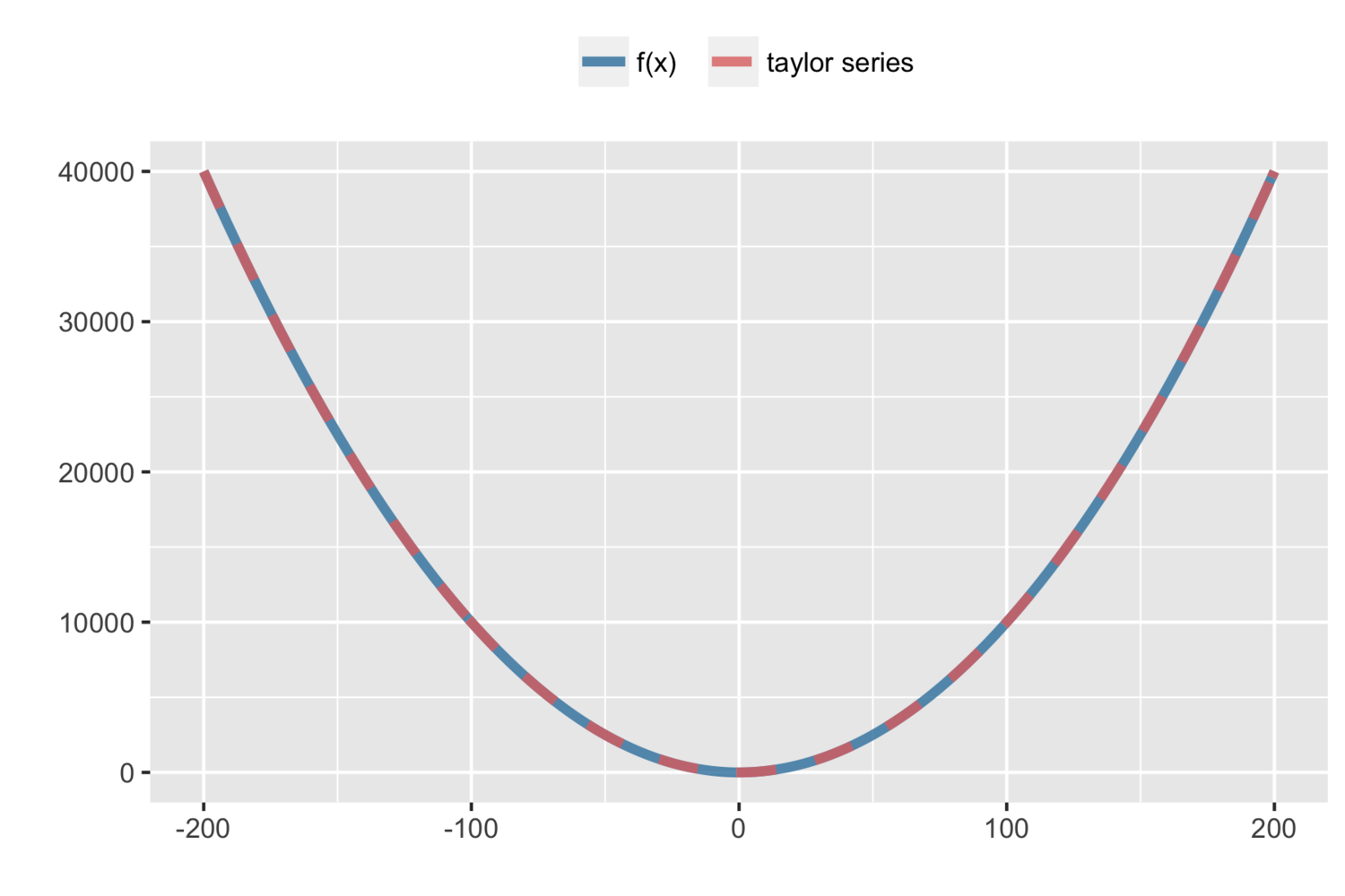
Recall the basic Taylor series expansion, where a function about a point \(a\) can be expanded into a (sometimes infinite) sum of terms, and using a finite number of these terms can serve as an approximation (often the first three terms are used, up to the second derivative).
$$ \begin{equation*} f(x) = f(a) + \frac{f’(a)}{1!}(x-a) + \frac{f’’(a)}{2!}(x-a)^2 + \frac{f’’’(a)}{3!}(x-a)^3 + … \end{equation*} $$
Say we have the basic parabola, \(y = x^2\). Expand around \(a = 2\) (here we could pick any value):
$$ \begin{align*} f(x) = x^2 \hspace{7mm} f’(x) = 2x, \hspace{7mm} f’’(x) = 2, \hspace{7mm} f’’’(x) = 0 \end{align*} $$
And therefore:
$$ \begin{align*} f(x) = x^2 = 2^2 + 2(2)(x-2) + \frac{2}{2}(x-2)^2 \end{align*} $$
A Laplace approximation is used to estimate any distribution (PDF) with a normal distribution. It uses the first three terms (quadratic function) Taylor series expansion around the mode \((\hat{x})\) of a function to approximate \(\log g(x)\) (the log simplifies differentiation):
$$ \begin{align} \log g(x) \approx \log g(\hat{x}) + \frac{\partial \log g(\hat{x})} {\partial x} (x-\hat{x}) + \frac{\partial^2 \log g(\hat{x})} {2 \partial x^2} (x-\hat{x})^2 \end{align} $$
The first derivative at the mode is zero, so the above expression simplifies, and if we say the estimated variance (based on curvature) is \(\hat{\sigma}^2 = -1 / \frac{\partial^2 \log g(\hat{x})} {2 \partial x^2}\), then we can re-write these expressions as:
$$ \begin{align} \log g(x) \approx \log g(\hat{x}) - \frac{1}{2\sigma^2} (x-\hat{x})^2 \end{align} $$
Which hopefully is beginning to look familiar! We can use this result to do a normal approximation. Taking the exponent and integral of both sides and moving out the constants:
$$ \begin{align} \int g(x)dx = \int exp[\log g(x) dx] \approx constant \int exp[ - \frac{(x-\hat{x})^2}{2\hat{\sigma^2}}]dx \end{align} $$
Using a Laplace approximation the distribution \(f(x)\) is approximately normal with mean \(\hat{x}\) which can be found by solving \(f’(x) = 0\), and variance \(\hat{\sigma}^2 = -1/f’’(x)\) at the mode. Not quite convinced? Here’s a quick example with \(\chi^2\) (cause it’s easy to differentiate by hand; the gamma terms in the denominator are just constants).
$$ \begin{align} f(x;,k) &= \frac{x^{(k/2-1)} e^{-x/2}}{2^{k/2} \Gamma\left(\frac{k}{2}\right)}, x \geq 0 \end{align} $$
$$
\begin{align}
\log f(x) &= (k/2 - 1) \log x - x/2
\end{align}
$$
$$
\begin{align}
\log f’(x) &= (k/2 -1)/x - 1/2 = 0
\end{align}
$$
$$
\begin{align}
\log f’’(x) &= -(k/2 - 1)/x^2
\end{align}
$$
$$
\begin{align}
\therefore \chi^2_k &\overset{LA}{\sim} N(\hat{x} = k-2, \hat{\sigma}^2 = 2(k-2))
\end{align}
$$
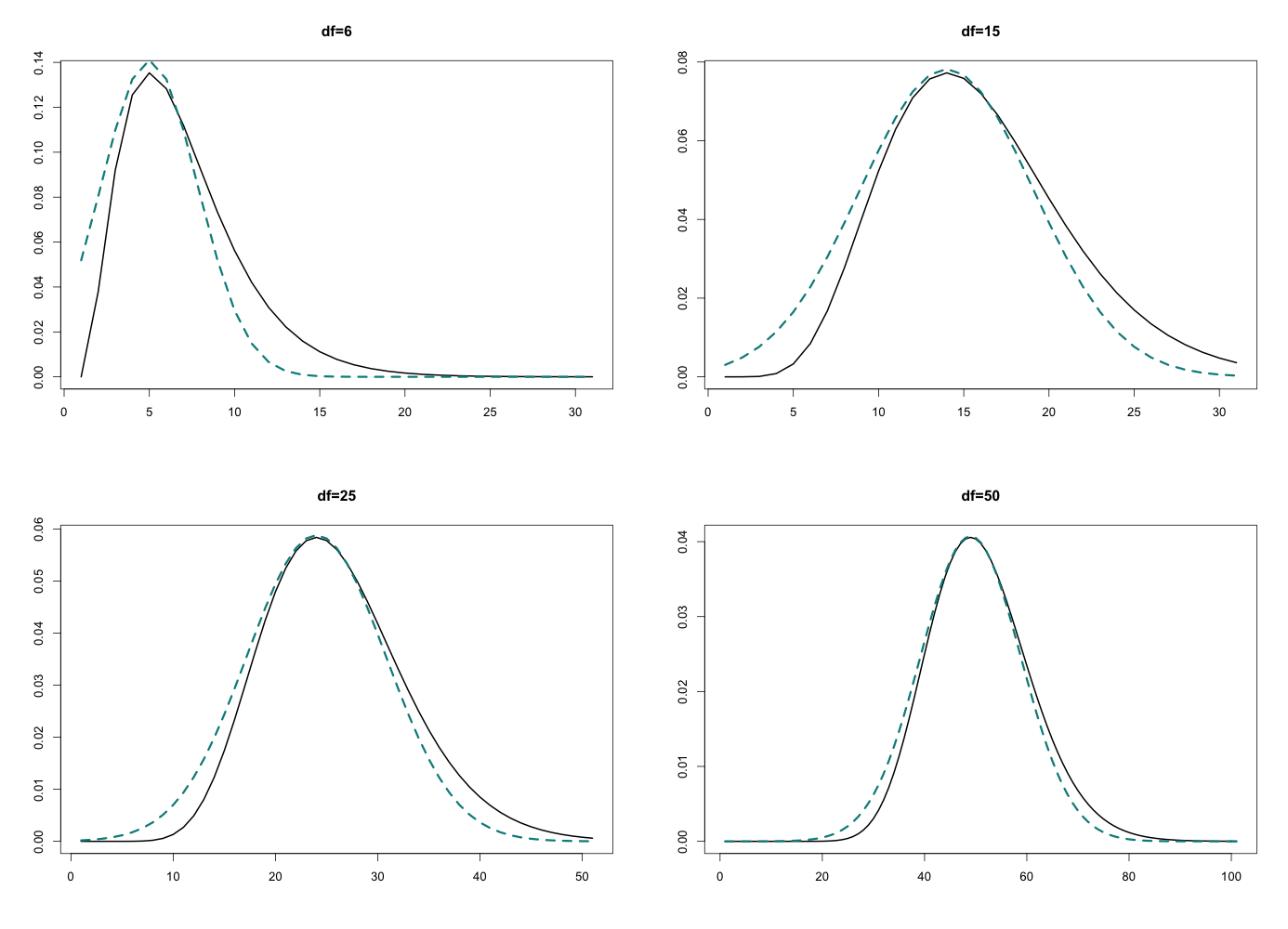
The approximation is clearly better when the degrees of freedom are higher (when the distribution more closely resembles a normal). This is a very simple univariate example, but the point is just to convince you that when things are approximately normal, this tends to work well. It extends to multivariate cases as you would expect, using the Hessian for curvature, and lots of math ensues…
We just covered a lot of different pieces, but what we want from our LGMs are the marginals for the elements of the latent field (e.g., regression parameters) and possibly some elements from hyperprior distributions (e.g., the correlation parameter in an autoregressive model, or the variance on a random effect) - we want to fit a hierarchical model!
$$ \begin{equation} p(x_j | \mathbf{y}) = \int p(x_j, \mathbf{\theta} | \mathbf{y}) d\mathbf{\theta} = \int p(x_j | \mathbf{\theta},\mathbf{y}) p(\mathbf{\theta} | \mathbf{y}) d\mathbf{\theta} \end{equation} $$
$$ \begin{equation} p(\theta_k | \mathbf{y}) = \int p(\mathbf{\theta}|\mathbf{y}) d\mathbf{\theta}_{-k} \end{equation} $$
And therefore the terms we need to approximate are: \(p(\mathbf{\theta}|\mathbf{y})\) and \(p(x_j | \mathbf{\theta}, \mathbf{y})\). The first term can be used to estimate all the marginals of interest for \(\mathbf{\theta}\) and is also needed to estimate the marginals for the latent field.
Recall from probability:
$$ \begin{align} p(b) &= \frac{p(a,b)} {p(a|b)} \end{align} $$
$$ \begin{align} p(b|c) &= \frac{p(a,b|c)} {p(a|b,c)} \end{align} $$
We can use this rule to rewrite our marginal distributions:
$$ \begin{align} p(\mathbf{\theta} | \mathbf{y}) &= \frac{p(\mathbf{x}, \mathbf{\theta} \mathbf{|} \mathbf{y})} {p(\mathbf{x} \mathbf{|} \mathbf{\theta}, \mathbf{y}) } \nonumber \end{align} $$
We can expand the numerator (details omitted) and use a Laplace approximation for the dominator, which is unknown:
$$ \begin{align} p(\mathbf{\theta} | \mathbf{y}) &\approx \frac{p(\mathbf{y|x,\theta}) p(\mathbf{x|\theta})p(\mathbf{\theta})} {\tilde{p}(\mathbf{x|\theta,y})} \bigg|_{x={x^*}(\theta)} = \tilde{p}(\mathbf{\theta|y}) \end{align} $$
Where \(x^*(\theta)\) is the mode of \(\mathbf{x}\) for a given configuration of \(\mathbf{\theta}\). Obtaining \(p(x_j | \mathbf{\theta}, \mathbf{y})\) uses the same logic, but is more complex because the dimensionality of \(\mathbf{x}\) is much larger.
The most obvious option is to use a normal approximation for \(p(x_j|\mathbf{\theta},\mathbf{y})\) directly, as we have already calculated this in the denominator above. This is very fast, but the assumption is too strong and results are often poor (these conditional distributions are often somewhat skewed or heavy tailed).
Alternatively, we can partition \(\mathbf{x} = [x_j, \mathbf{x}{-j}]\) and use the Laplace approximation for each element in the latent field \(\mathbf{x}\):
$$ \begin{align} p(x_j | \mathbf{\theta,y}) \propto \frac{p(\mathbf{x,\theta |y})}{p(\mathbf{x}{-j} | x_j, \mathbf{\theta, y})} \propto \frac{p(\mathbf{\theta})p(\mathbf{x|\theta})p(\mathbf{y|x})}{p(\mathbf{x}_{-j} | x_j, \mathbf{\theta, y})} \end{align} $$
This approach works very well, because the conditionals \(p(\mathbf{x_{-j}} | x_j, \mathbf{\theta, y})\) are often close to normal, but is computationally more expensive.
The third option (default in INLA software) uses a simplified Laplace approximation (sort of a compromise between the two), which is very computationally efficient and the approximation is still very good. It uses a Taylor’s series expansion up to the third order of both the numerator and the denominator for estimating \(p(x_j|\mathbf{\theta,y})\).
Either of the other two options can also be used in INLA. I personally fit the models with the approximations to begin, because it’s so wonderfully fast. The results ballpark but are often noticably different from say using MCMC (or the truth if you’re doing a simulation). So I do some basic building and validation with the approximation, then use the simplified or full Laplace for the final models. I’ve never personally observed a scenario where I can distinguish meaningfully between the simplified and full Laplace.
The INLA algorithm uses Newton-like methods to explore the joint posterior distribution for the hyperparameters \(\tilde{p}(\mathbf{\theta|y})\) to find suitable points for the numerical integration:
$$ \begin{align} \tilde{p}(x_j|\mathbf{y}) \approx \sum_{h=1}^H \tilde{p}(x_j|\theta^*_h,\mathbf{y}) \tilde{p}(\theta^*_h|\mathbf{y}) \Delta_h \end{align} $$
And now we can get the gist of what INLA is doing!
Integrated: Using numerical integration
Nested: Because we need \(p(\mathbf{\theta | y)}\) to get \(p(x_j | \mathbf{y})\)
Laplace approximations: The method used to obtain parameters for the normal approximation
2011 research by Finn Lindgren and others presented a stochastic partial differential equation (SPDE) approach to INLA that allows for more realistic spatial modelling across large geographic areas that have curvature in the surface for point data, allowing for continuous covariance functions. I won’t discuss this today, but may do a future post on SPDEs. If you’re just starting to learn about INLA, unless the SPDE stuff is the only part you’re interested in, I would recommend learning the basics first. Stochastic calculus isn’t something most of us applied types use every day.
I know that was a lot of information - but I’ve actually barely scratched the surface! I recommend looking at the 2009 original INLA paper (see the references). For now, let’s switch to seeing how R-INLA code looks and how the output compares to using MCMC in some simple examples.
R-INLA relies on a stand-alone C library (GMRF) and therefore is not on CRAN, but you can get all the info from http://www.r-inla.org .
I’m going to go through two very simple examples of MCMC using rjags and INLA
using R-INLA.
$$ E(y_i|x_i) = \alpha + \beta x_i $$
Simulated data in R
N <- 100 # 500, 5000, 25000, 100000
x <- rnorm(N, mean = 6, sd = 2)
y <- rnorm(N, mean = x, sd = 1)
data <- list(x = x, y = y, N = N)
JAGS code
model <- function() {
  for(i in 1:N) {
    y[i] ~ dnorm(mu[i], tau)
    mu[i] <- alpha + beta * x[i]
  }
  alpha ~ dnorm(0, 0.001)
  beta  ~ dnorm(0, 0.001)
  tau   ~ dgamma(0.01, 0.01)
}
params <- c("alpha", "beta", "tau", "mu")
jags(
  data = data,
  param = params,
  n.chains = 3,
  n.iter = 50000,
  n.burnin = 5000,
  model.file = model
)
INLA code
inla(y ~ x,
  family = "gaussian",
  data = data,
  control.predictor = list(link = 1)
)
| n | rjags | r-inla |
|---|---|---|
| 100 | 4.19 | 0.176 |
| 500 | 18.141 | 0.359 |
| 5000 | 381.573 | 2.787 |
| 25000 | 2203.679 | 13.27 |
| 100000 | 8873.836 | 52.787 |
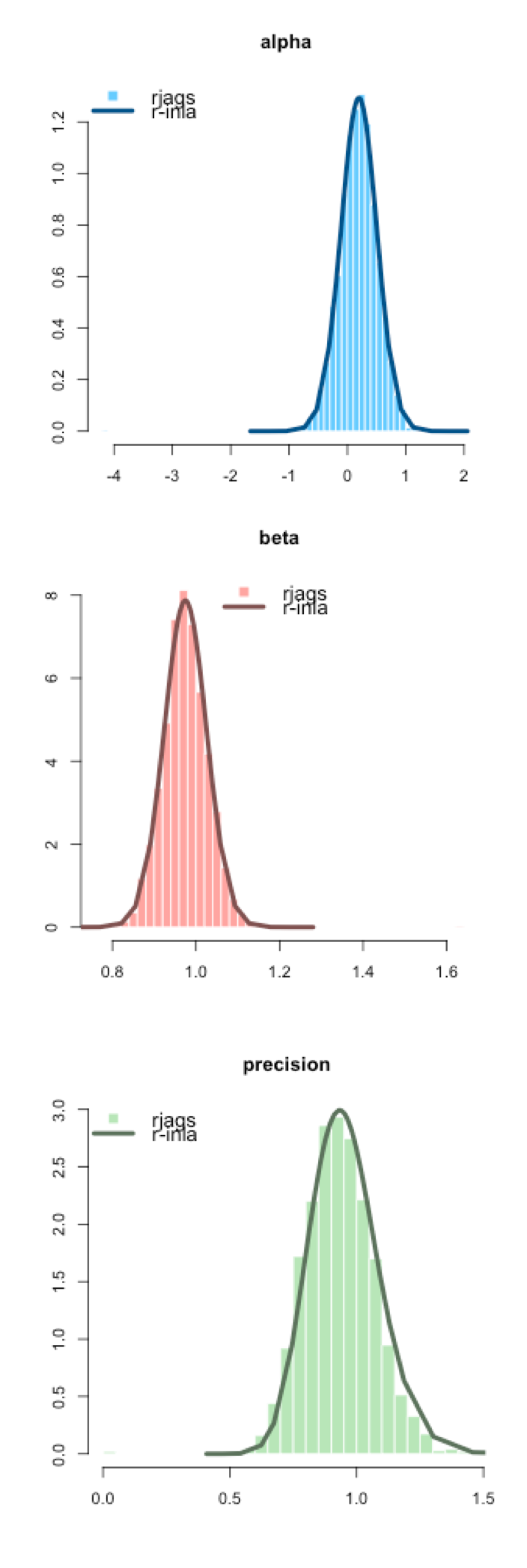
INLA generates a posterior density rather than a simulated empirical distribution like MCMC. You can see in the figure to the right how similar the distributions are from JAGS (the histogram) and INLA (the density curve) for these three parameters.
It was easy here, but sometimes it can be hard to know what the default INLA priors are and they can play a big role, especially when the dataset is small. If you’re comparing MCMC and INLA, before assuming that the INLA approximation has failed, I highly recommend confirming the priors you are using are the same. Sometimes INLA defines priors on the logit scale (for example).
Even for this simple example, as the sample size increased the time savings for R-INLA vs JAGS was remarkable.
$$ E(y_i|x_i) = poisson(\mu_i) $$ $$ log(\mu_i) = \alpha + \beta x_i + \nu_i $$ $$ \nu_i \sim N(0,\tau_\nu) $$
Simulated data
N <- 100 # 500, 5000, 25000, 100000
x <- rnorm(N, mean = 5, sd = 1)
nu <- rnorm(N, 0, 0.1)
mu <- exp(1 + 0.5 * x + nu)
y <- rpois(N, mu)
JAGS code
model = function() {
  for(i in 1:N) {
    y[i] ~ dpois(mu[i])
    log(mu[i]) <- alpha + beta * x[i] + nu[i]
    nu[i] ~ dnorm(0, tau.nu)
  }
  alpha  ~ dnorm(0, 0.001)
  beta   ~ dnorm(0, 0.001)
  tau.nu ~ dgamma(0.01, 0.01)
}
params model = function() {
  for(i in 1:N) {
    y[i] ~ dpois(mu[i])
    log(mu[i]) <- alpha + beta*x[i] + nu[i]
    nu[i] ~ dnorm(0, tau.nu)
  }
  alpha  ~ dnorm(0, 0.001)
  beta   ~ dnorm(0, 0.001)
  tau.nu ~ dgamma(0.01, 0.01)
}
params <- c("alpha", "beta", "tau.nu", "mu")
jags(
  data = data,
  param = params,
  n.chains = 3,
  n.iter = 50000,
  n.burnin = 5000,
  model.file = model
)
INLA code
nu <- 1:N
inla(y ~ x + f(nu, model = "iid"),
  family = "poisson",
  data = data,
  control.predictor = list(link = 1)
)
I didn’t show the distributions here but the parameter estimates were comparable. The time savings is really remarkable again. In my PhD, I proposed a multivariate (multiple outcome) model for forecasting and without the INLA approach, it wouldn’t have been a practical model for the public health application I was working on, as the model had to be re-fit each day. I’ll reference my paper about that model here as well. Although what I do now tends to be less complex, I still like using INLA for a lot of my Bayesian work.
| n | rjags | r-inla |
|---|---|---|
| 100 | 30.394 | 0.383 |
| 500 | 142.532 | 1.243 |
| 5000 | 1714.468 | 5.768 |
| 25000 | 8610.32 | 30.077 |
| 100000 | got bored after 6 hours | 166.819 |
The only thing I prefer about MCMC code, besides the more intuitive theory, is the syntax of BUGS/JAGS vs INLA. While INLA looks nice because it’s similar to the glm function in R, sometimes the priors are too hidden for my liking. I find the BUGS code really highlights the hierarchical structure of the models in a way that is good for teaching and learning.
Do you use Bayesian models in your applied research or work? Do you write your own MCMC or use Bugs, Jags or Stan? Have you tried INLA?
Find out more about our R training courses by contacting us at contact@precision-analytics.ca !
Rue H, Martino S, Chopin N. 2009. “Approximate Bayesian inference for latent Gaussian models by using integrated nested Laplace approximations.” Journal of the Royal Statistical Society: Series B (Statistical Methodology) 71(2): 319-392.
Bolin D, Lindgren F. 2011. “Spatial models generated by nested stochastic partial differential equations, with an application to global ozone mapping.” The Annals of Applied Statistics 523-550.
Morrison KT, Shaddick G, Henderson SB, Buckeridge DL. 2016. “A latent process model for forecasting multiple time series in environmental public health surveillance.” Statistics in Medicine 35(18): 3085-3100.
Edit Thanks to @jim_savage for catching a typo! (wrong family in the 2nd INLA model)