
As a Data Scientist at Precision Analytics, I have had the good fortune to meld my background in epidemiology and biology with …
An introduction to decision tree theory
At Precision Analytics, we focus on finding the best tools to address the scientific question in front of us and machine learning is one useful option. Decision trees are a good place to start learning about machine learning because they offer an intuitive means of analyzing and predicting data. We wanted to showcase an application of decision trees in heath and related sciences, though the content will be equally relevant to other disciplines.
This series is meant to provide sufficient explanation of theory, analysis steps, and code to be able to confidently implement a decision tree analysis while, most importantly, understanding the why and how of all the steps taken. Accordingly, we will be bringing a three-part series that will cover:
- Part 1: Introduction to decision tree theory (below)
- Part 2: Implementation of a decision tree analysis, including hyperparameter tuning
- Part 3: Comparison of a standard decision tree and related ensemble models (random forest)
Decision tree analysis is a supervised machine learning method that are able to perform classification or regression analysis (Table 1). At their basic level, decision trees are easily understood through their graphical representation and offer highly interpretable results. Some examples relevant in the field of health are predicting disease stage through clinical history, laboratory tests and biomarker levels, or predicting antibody concentration in response to vaccination based on patient and vaccine characteristics.
| Prediction type | Outcome type | Outcome example |
|---|---|---|
| Classification | Categorical | Survival (died or survived) following coronary artery bypass graft surgery |
| Regression | Continuous | Low density lipoprotein levels in heart disease patients on different treatment regimens |
Table 1 Types of decision trees, associated outcome types, and examples.
A tree begins with a root node which is split into two branches; each subsequent split occurs at an intermediary node, also sometimes called a decision node. The tree ends with the terminal or leaf nodes and any subset of connected nodes is referred to as a sub-tree (Fig 1).
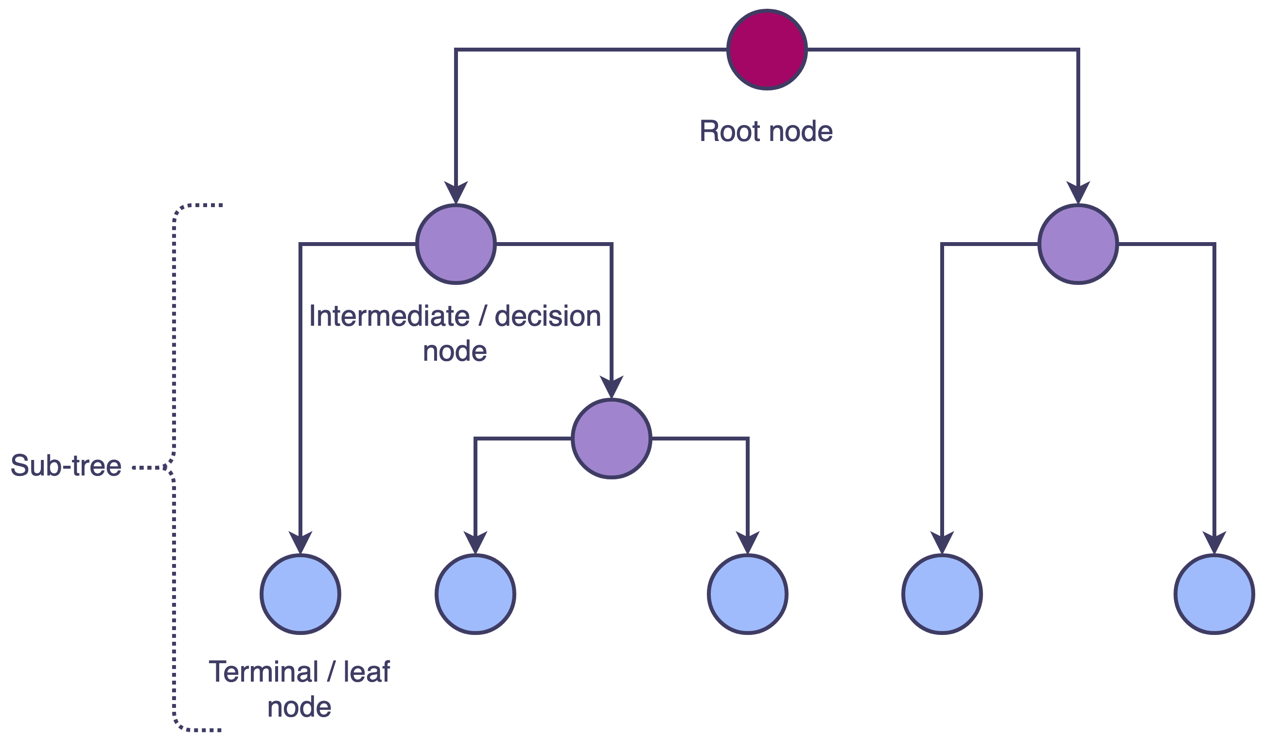
Fig 1. Decision tree structure where each node split results in two branches. The initial split is made at the root node, subsequent splits are made at intermediate/decision nodes and the tree ends with unsplit terminal/leaf nodes. A subset of connected nodes is a sub-tree.
Decision trees are most commonly used for prediction. By way of following the path determined by the decision split at each node, a new observation can be predicted to belong to one of k terminal nodes and from there obtain its predicted value.
In classification, the predicted outcome class will be the class with the highest proportion of training observations in that terminal node (Fig 2A).
A regression tree, on the other hand, will predict a numerical value for the outcome. Each terminal node is assigned the mean of the training observations’ outcome values in that node. Therefore, the predicted value of an observation is the mean outcome value in the terminal node to which it belongs (Fig 2B).
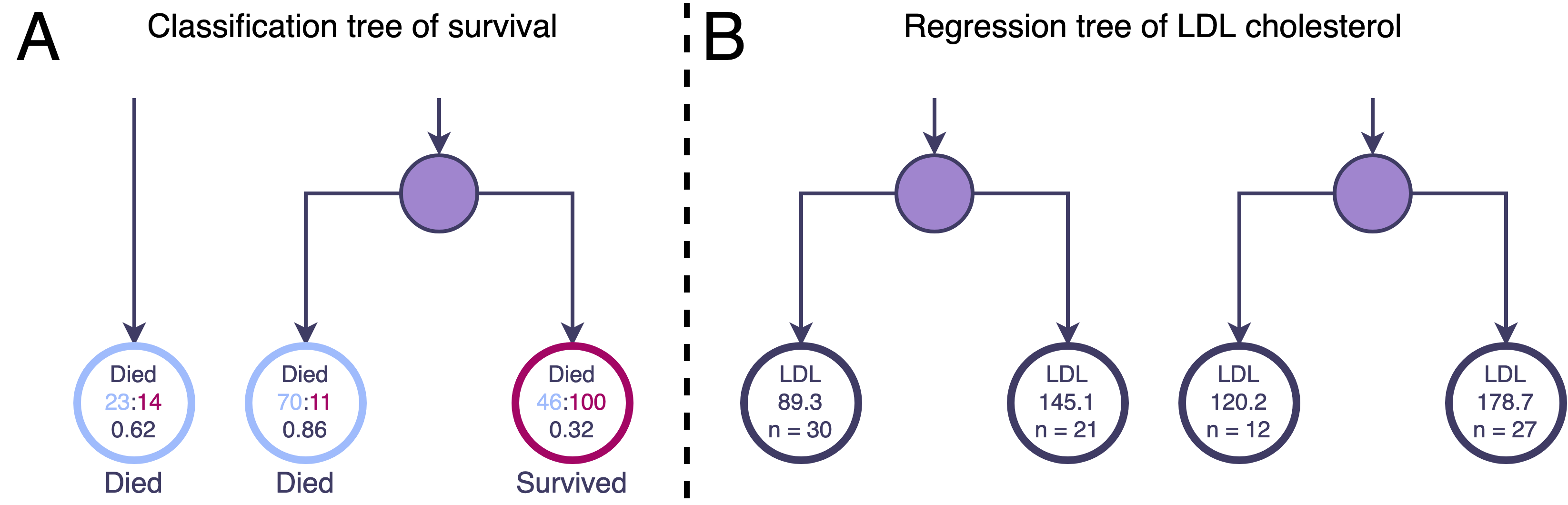
Fig 2. Zoom in on some terminal nodes of imagined classification and regression decison trees. A. The classification terminal nodes give the ratio and corresponding proportion of training observations with the outcome Died (levels of Died and Survived). The class with the highest proportion will be the one assigned to new observations falling into that node. For example, the two leftmost nodes in panel A have a greater number of observations with outcome Died than Survived (23 v. 14, and 70 v. 11) and so take the value Died whereas the rightmost node contains more observations that Survived and so takes that class value. B. The regression terminal nodes give the mean value of the outcome low density lipoprotein (LDL) for the observations in those nodes. A new observation belonging to any of these terminal nodes will be predicted to have the corresponding LDL value. For example, the two left terminal nodes share an intermediate parent node. A new observation falling into the left child node will have a predicted LDL of 89.3 mg/dL compared to a new observation falling into the right child node with a predicted LDL of 145.1 mg/dL.
It wouldn’t be feasible to compute every possible tree based on all permutations of node splits. Instead, decision trees implement what is known as recursive binary splitting. Binary splitting means that each node is split with a decision from one predictor that can be represented in a binary way.
For example, \(X_i < a\), where \(X_i\) is a predictor and \(a\) is some constant, can be applied as a logical true/false test to each observation in a node.
Recursive means that the binary splitting assessments are applied to the results of the previous split until some stopping criteria are met.
This approach is also called top-down and greedy. Top down because the entire data set (at the root node and later the data belonging to each intermediate node) is assessed and split as opposed to examining subsets of the data. And greedy because, at each step, the optimal split is made for that step without taking into account potentially more advantageous splits further down the tree.
Quite generally, each predictor and each cutpoint of each predictor is considered at every node splitting step. Categorical predictors, for example smoking status, are supported without requiring conversion to dummy variables. A cutpoint for a categorical predictor is defined as belonging to one or more of its classes. For this reason, ordered factors can often be more informative in decisions than standard factors. The predictor and corresponding threshold that most reduces the error in the tree at that step is selected. Many different measures for error, or risk, can be used.
For a regression tree, often the residual sum of squares is evaluated for the parent node and both potential child nodes. The child node RSS are summed and compared to the value for the parent node.
For classification trees, the Gini index or a measure called entropy are among those applied. The Gini index is often called a measure of purity and it and the entropy measure are both minimized when almost all of the observations of a node belong to the same outcome class. The predictor/cutpoint providing the greatest purity in the child nodes will be selected.
Observations with missing predictor values are not always excluded from the analysis. Splits involve one predictor at a time so a tree may grow without ever needing to evaluate an observation’s missing data.
If an observation with a missing value for the best predictor is present in a given node, a surrogate predictor, i.e. the best non-missing predictor for those observations, is selected in the same way (RSS, Gini index, etc). This method allows the retention of observations with missing data; however, it can affect both the interpretability of the model results and its performance in prediction.
As previously mentioned, a tree will grow until some criteria are met. A standard criterion would allow growth until each node contains less than a minimum number of observations required for further splitting. Once a node contains less than the minimum it will become a terminal node.
If left to grow, the potentially large and sprawling tree is likely to overfit the data. Overfitting , in simple terms, means that the model has learned the training set too well and may not generalize effectively to the test data or other external data sources resulting in poor prediction performance.
Pruning is used to remove nodes or entire sub-trees and can be approached in different ways. A simple means is to assign a maximum depth to which a tree can grow. Another common method is to increase that minimum number of observations in a node before it can be split.
Alternatively, cost-complexity pruning assigns a non-negative cost to each terminal node in the tree. In this way, the error increases with increasing complexity of the tree. When the cost complexity value is zero, the tree will be equivalent to its maximum size. Increasing the cost results in minimizing error through a smaller less complex tree as branches are removed in a nested fashion.
Each of these hyperparameters , tree depth, minimum node observations, and cost complexity, can be tuned to obtain the best fit for model performance. Tuning can be done on a validation set or alternatively using cross validation .
Check out Part 2 of our decision tree series , where we implement a decision tree in R using the tidymodels ensemble of packages.
Find out more about our R training courses by contacting us at contact@precision-analytics.ca !
James, G., Witten, D., Hastie, T., & Tibshirani, R. (2013). An introduction to statistical learning: With applications in R. Springer Texts in Statistics. Springer Science+Business Media New York.
Therneau, T., & Atkinson, E. (2018, April 11). An introduction to recursive partitioning using the RPART routines. The Comprehensive R Archive Network. Retrieved October 2021, from https://cran.r-project.org/web//packages/rpart/vignettes/longintro.pdf .