In my last post , I showed how makeup brands’ prices and ratings correlated visually. For this post, I decided to continue my exploration using k-means clustering, an unsupervised machine learning method. There are plenty of online tutorials on k-means, but briefly, k-means is a technique that allows us to find patterns (or clusters) in data. In the simplest and typical application, we can use continuous variables to group together observations, in this case makeup products, to detect any patterns across our observed variables, price and ratings.

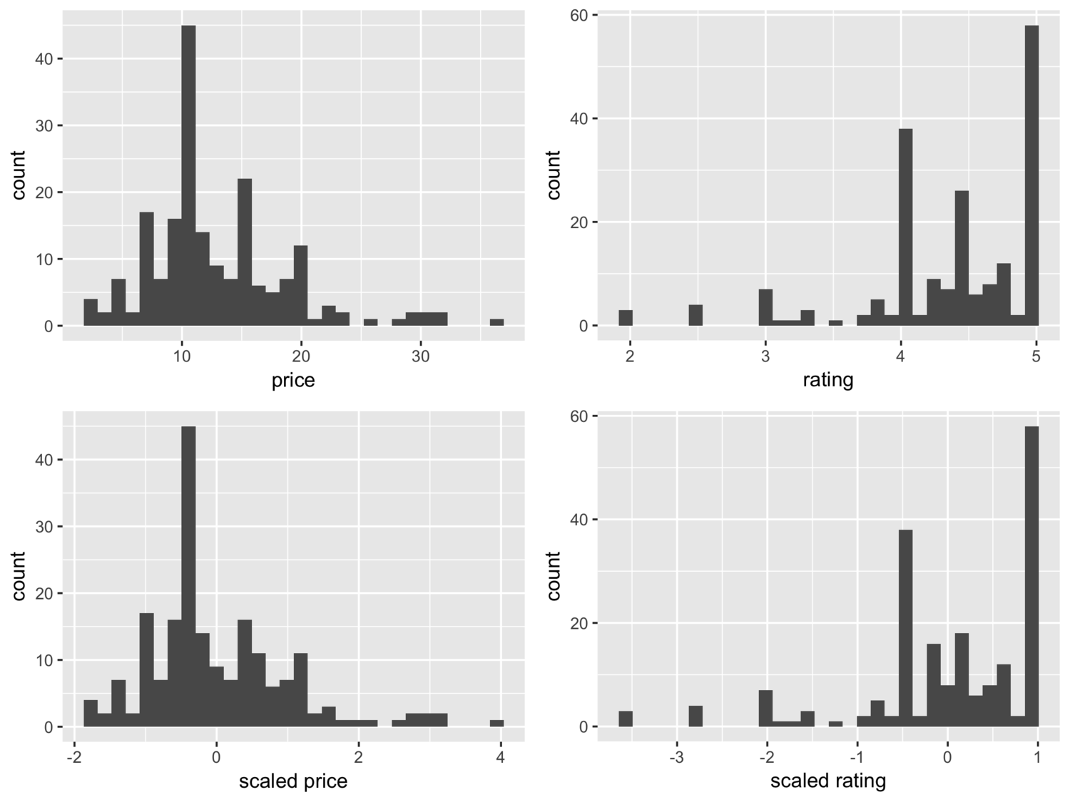
I first began by scaling my data, which means that each column is transformed to a common scale (z-score) with an approximately normal distribution. For each variable, the mean is subtracted from each value and divided by the standard deviation. Initially, neither price nor rating is normally distributed. After scaling, the interpretation for each respective value is the number of standard deviations away from the overall mean.

On its own, k-means does not tell us very much about how well our model is doing at fitting the data. We need to have an a priori idea of how many clusters we expect to see, or be willing to experiment by looking at different clustering solutions. How k-means works is that it starts by randomly assigning k (the number of clusters we’ve pre-specified) data points to act as the cluster’s centroid. These centroids will serve as a sort of anchor around which the k-means will try minimize the distance between neighbouring points. The algorithm then calculates the average distance of all the points in a given cluster, and then moves the centroid to that centre location. The process of iteratively moving the centroid stops when cluster memberships ceases to change.

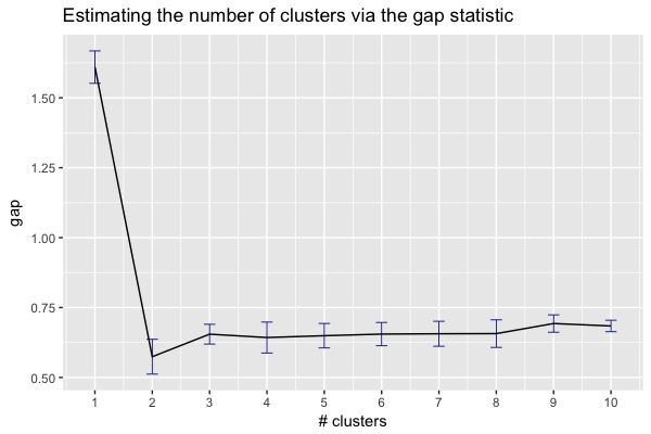
We need to rerun k-means using a different number of clusters to see which solution (i.e. the number of cluster) best fits our data. There are several approaches to model selection with k-means, but a common way to determine the optimal number of clusters is to compute the gap statistic. The gap statistic compares the pooled within-cluster sum of squares with a simulated uniform distribution obtained by resampling the data. The goal is to maximize the gap statistic, while choosing a parsimonious model. In other words, we want a large gap statistic with the fewest number of clusters.

I ran a function that computes the gap statistics automatically using different numbers of clusters, which is also known as a scree plot. From the plot we can see that the gap statistics peaks at a single cluster, and then tapers off. This is a sign that there are no discernible clusters in our data!

I wanted to share this analysis to illustrate an important point. Data does not always follow our assumptions. Many times, we can conduct an analysis and discover that the things we were hoping to find (beautifully evident clusters with immediately discernible meaning) aren’t always present. A null finding is still a finding and we as researchers and analysts shouldn’t get discouraged when things don’t turn out the way we expected.

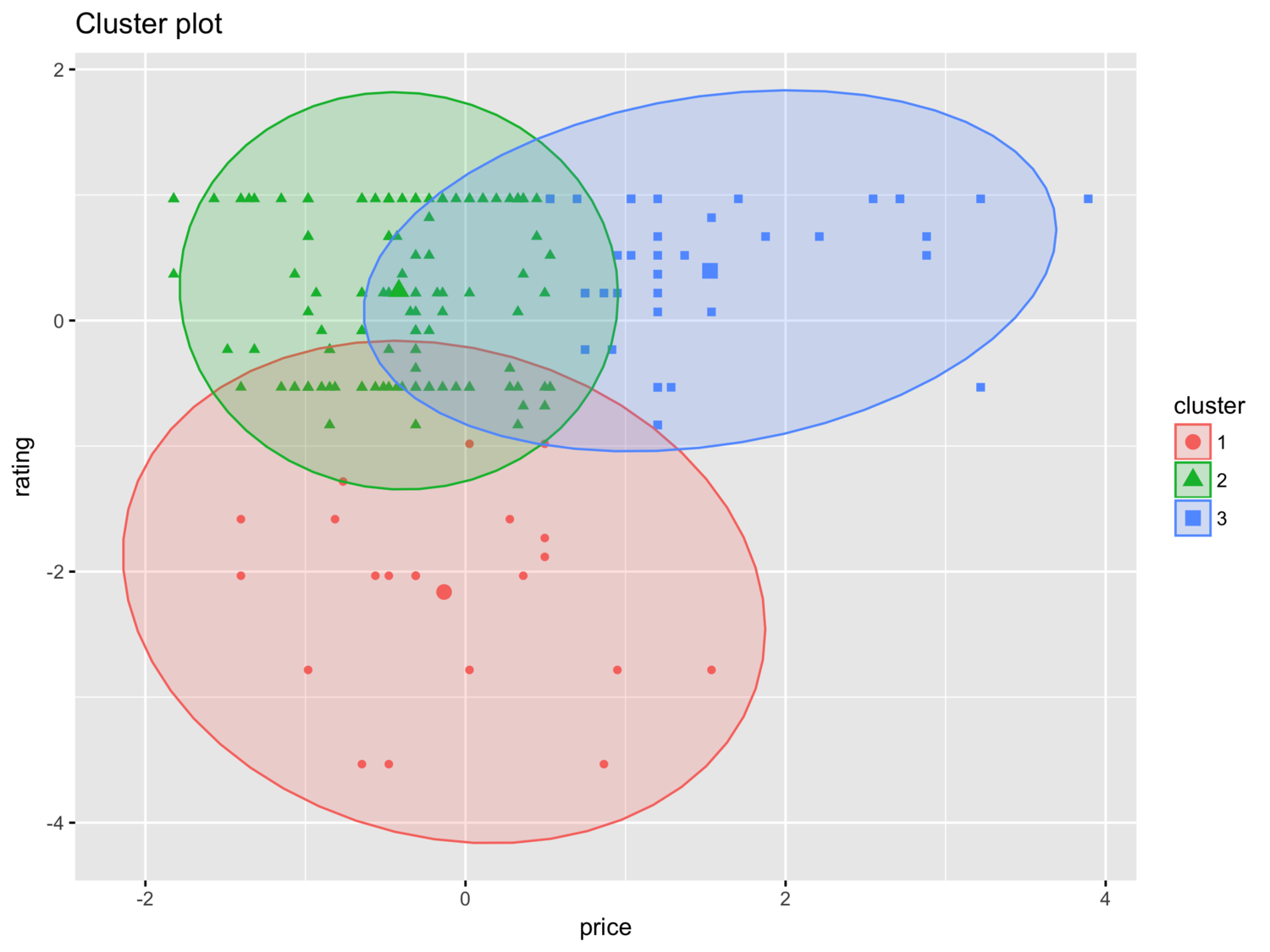
For the purpose of this blog post, I’ll pretend as though we found that there were three clusters in our data. Recall that we scaled the data prior to the analysis so the x- and y-axis represent standard deviations away from the mean. The plot is not showing us anything ground breaking. There are 39 products in first cluster, 136 is the second and 22 in the third. Since we only have two variables, our interpretation of the plot is pretty straightforward. If we were going to assume a 3-cluster solution, close to 70% of products would fall in the “low price, decent ratings” category.

If I were doing this analysis in real life, I wouldn’t give up here. Since our data shouldn’t be clustered, I’d explore other options: 1) find more data, and/or 2) change my approach.